Ok, so what's wrong with the confidence intervals in this preprint? Well they publish a confidence interval on the specificity of the test that runs between 98.3% and 99.9%, but only 1.5% of all the tests came back positive! 1/

That means that if the true specificity of the test lies somewhere close to 98.3%, nearly all of the positive results can be explained away as false positives (and we know next to nothing about the true prevalence of COVID-19 in Santa Clara County) 2/

They report a 95% confidence interval for the prevalence of COVID-19 in Santa Clara County that runs from 2.01% to 3.49% though! That seems oddly narrow, given that they have already shown that it is within the realm of possibility that the data collected are all false positives!

What went wrong here? I think the key lies in their explanation of how they propagated the uncertainties presented. By first upweighting according to the demographics, and then adjusting for specificity, they understated the impact of the latter.

By upweighting first by demographics, they artificially increased the number of positive tests observed. With this larger number, suddenly the specificity issues raised earlier (a possible false positive rate of 1.7%) didn't matter quite so much.

What happens though if we reverse the order of the uncertainty propagation though? Let's first take into account the specificity of the test, and then after that, let's reweight the samples by age/sex/race.

I'm no expert on confidence intervals for these surveys, but here's a pretty reasonable strategy I came up with for computing one. Let's start by actually coming up with a representative set of possible specificities for our test.

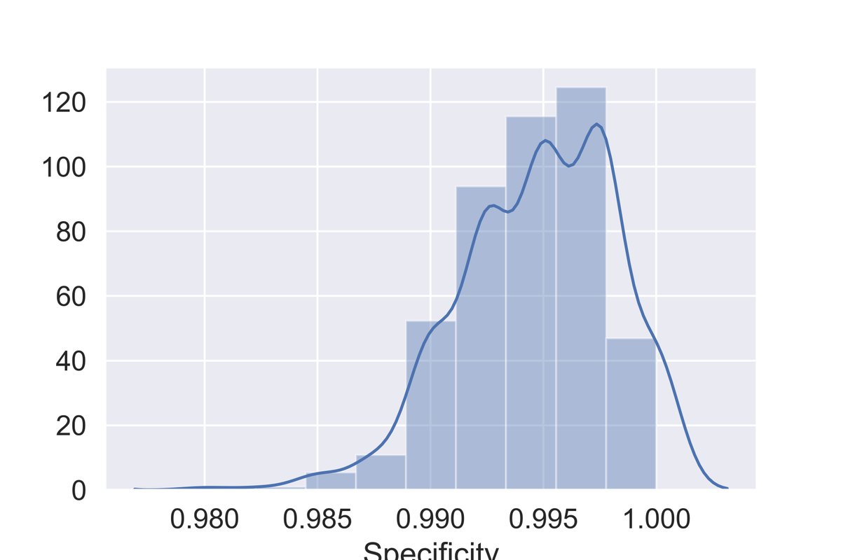
Rather than saying we have a confidence interval for our specificity between 98.3% and 99.9%, let's actually come up with numbers drawn from the probability distribution over specificities. To accomplish this, we can apply the bootstrap.

Now that we've used the bootstrap to come up with a set of guesses for the specificity of our test, we now bootstrap the actual observations. For each bootstrap sample (you can think of each as a redo of the study), we can evaluate the effect of the uncertain specificity.

To be more concrete, for each bootstrap sample, we compute the likely true positive rate for each "guess" of the test specificity that we had come up with in the prior bootstrap. Collecting every true positive rate in an array (and repeating this for all samples) gives us an...

estimate of how specificity affects our estimate of the true positive rate including both uncertainty in the test specificity and uncertainty in the sampling (i.e., the actual number of positives observed).

This whole time, for the sensitivity, I've assumed the worst-case (at least for computing a lower bound on the true positive rate): a 73% sensitivity rate corresponding to the lower bound on their 95% CI for the test's sensitivity.

So, what does the final confidence interval look like? Well the 95% CI on the true positive rate (the proportion of truly positive people in Stanford's study) runs from 0.5% to 2.8%. Adjusting for demographics to get an estimate of the county prevalence...

will increase that lower bound to something like 1% (far below the CI reported in the paper) and corresponding to a substantially higher mortality rate (at least 2x the upper bound and this is with conservative estimates on the test's sensitivity).

If we just plug in the expected sensitivity of the test, the upper bound on the mortality rate estimated in the Stanford study rises above 1%!

I'll attach pretty plots conveying all of this to this thread soon (thanks @HNisonoff and @lbronner for the help!), but I hope this conveys something useful to the people who have stuck with me and read all of this.

Assuming a sensitivity of 72%, this is what the histogram of possible true positive rates are. 95% CI: [0.2, 2.4]

This is what the range of possible specificities looks like. 95% CI matches the paper's estimate.

If any of you are interested in seeing how this all works and/or playing with this application of the bootstrap, check out https://github.com/jjcherian/medrxiv_experiment. Thanks to @HNisonoff for cleaning up and rewriting my code to make it readable for anyone not named me!

And thanks to @lbronner for adding the instructions on how to install everything!