The results of my #tweetorial poll were pretty clear: from over 350 votes, 38% of you want to know about causal survival analysis. So, pull up a chair and let’s talk time-to-event!

First things first, what do we mean by causal survival analysis?

An answer to the question: How would the average time to event have differed if everyone had received some exposure, versus if everyone had received some other exposure?

We can measure that difference between in time to event in many different ways. I prefer survival curves with risk differences at the end of follow-up, adjusting for baseline and time-varying confounding.

Hazard ratios are also an option but b/c of how they compare instantaneous risksets, they might not actually answer our *causal* question (even if we can address confounding!).

The details need their own tweetorial, but the curious can read more here https://www.ncbi.nlm.nih.gov/pmc/articles/PMC3653612/

Before deciding on an analysis, we need to figure out what kind of exposure we have.

The are two main categories:
(A) exposure happens once
(B) exposure happens repeatedly

If exposure happens once (A), then it’s a “point exposure”. An example of this is might be comparing two different surgical techniques, where baseline is time of surgery and exposure is the technique used.

If exposure happens repeatedly (B), then it’s a “sustained exposure”. An example be taking statins everyday versus taking placebo everyday.

We’ll start by talking about point exposures, the simplest of whcih is randomization.

In the causal diagram, randomization happens once & influences survival(Yt) at every time.

We can estimate the intention-to-treat effect with several different survival analysis approaches

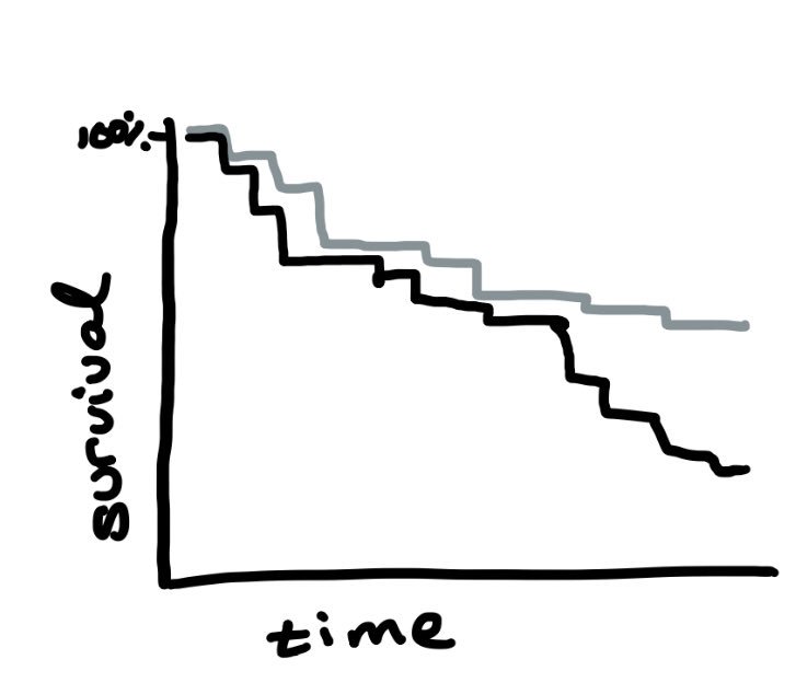
The simplest way to estimate the effect of randomization on time to event is with a Kaplan-Meier curve: it starts at 100% survival for each arm and decreases as people have the event.

In a trial w/ no loss to follow-up, this is is causal for *assignment* to treatment

There are two problems with Kaplan-Meier curves though: (1) when there is loss to follow-up, KM curves assume it’s random; and (2) KM curves are unadjusted, so they can be misleading when there is confounding.

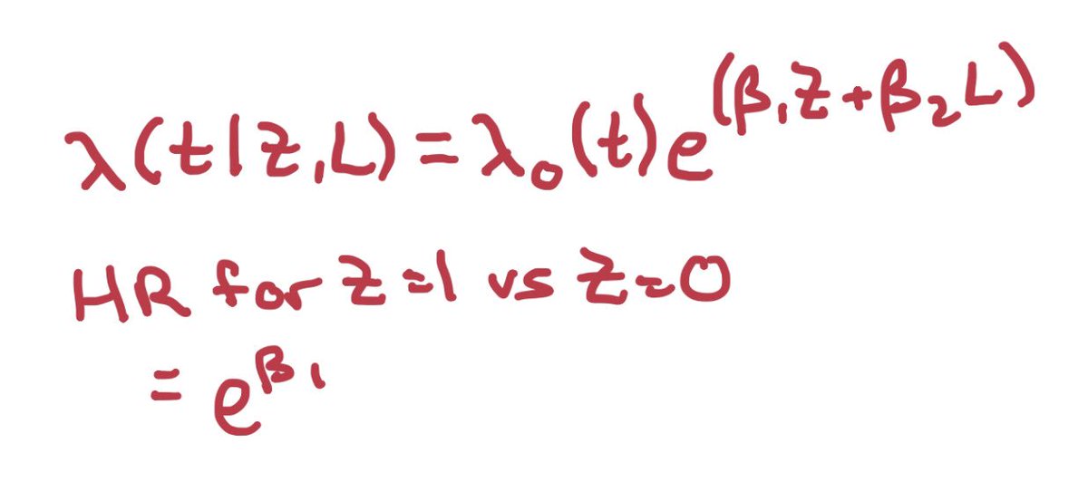
The next step up is time-to-event regression, the most common of which is a Cox proportional hazards model. This allows us to control for baseline confounding, but still assumes random loss to follow-up, & now assumes hazard ratio is constant over time (aka proportional hazards).

Cox models are easy to use, but don’t really give us much information. The hazard ratio is *at best* interpretable as the causal effect holding all covariates constant, and at worst isn’t interpretable causally at all, even if the 2 strong assumptions above are correct.

So, we have 2 problems: (1) we would like a more interpretable measure, while also adjusting for confounding (but without having to “hold them constant”); (2) we would like to be able to adjust for non-random loss to follow-up (ie informative censoring).

We can solve problem (1) by using a regression model which estimates the baseline rate of events (hazard); and we can solve problem (2) by using a method which allows us to adjust for time-varying covariates (since loss to follow-up happens over time and not just at baseline).

Even better, we can solve both problems at the same time! There’s more than 1 way, but I’m going to talk about the one I think is easiest to implement: inverse probability weighting of a pooled logistic regression model, with standardization over baseline covariates.

That sounds like a lot but it’s worth it. The first step is to decide what confounders you need. For a point exposure, we only care about baseline confounders(L0), but for loss to follow-up (Ct) we also need time-varying confounders (Lt).

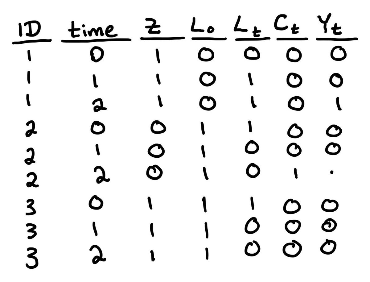
Lets assume you’ve chosen some of each. The next step is to make sure your data is in “long format”. That is, one row for each person for each time point. It should look something like this

Now we’re ready to create our inverse probability of censoring weights: we fit a model for the probability of being uncensored at each time, given baseline & time-varying covariates; a 2nd model without time-varying covariates; and use these to calculate the weights(SW)

The models we fit are pooled logistic regression models, because our intercept term (β0) is time-varying (β0,t). In practice that means we’ve added our time variable to the model, probably with a spline or other flexible form

So, let’s recap: we run 2 regression models, generate predicted probabilities for each person at each time, and then use them to calculate stabilized inverse probability of censoring weights (SW) using the formula below

Next, we estimate the time-to-event with a pooled logistic regression model for death, given randomization, and baseline covariates, and weight the model using our new weights.

Now, we have solved problem (2): we have a model that adjusts for non-random loss to follow-up. If we want, we can use the coefficient on Z to get the average hazard ratio, holding the covariates constant.

But we also wanted better interpretability! So let’s not stop here!

The final step is standardization: we make 2 copies of our dataset where everything is the same except in one copy we give everyone Z=1, and in the other we give them all Z=0.

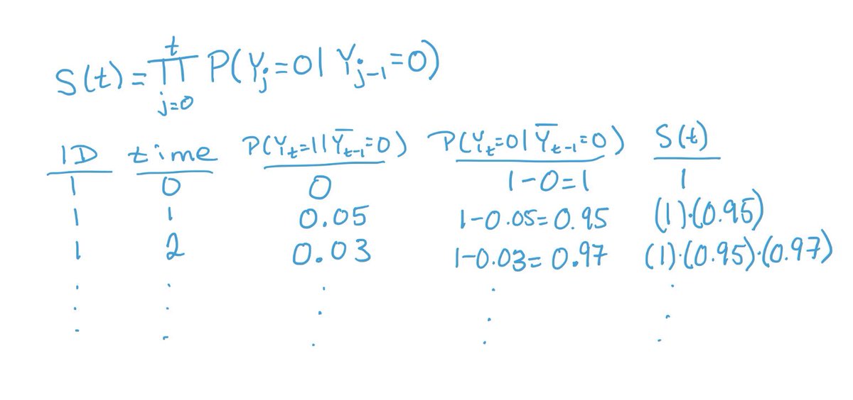
Then, we use our weighted pooled regression model coefficients to estimate predicted event probabilities at each time for each person. And finally, we use those predictions to generate survival estimates, S(t), using the product limit method you’ve likely used for KM curves.

We can use the survival estimates to plot survival curves, or calculate risks at the end of follow-up and get risk differences. These are interpretable as average treatment effects (assuming we picked the right covariates & a good model for time in our regressions!).

That’s all we need for simple *point* exposures, but sometimes our point exposures aren’t simple (for example when people can get treated anytime within a window or “grace period”) and other times we have sustained exposures.

Sustained exposures can be two kinds: static or dynamic. A static strategy is one which doesn’t depend on an individual’s characteristics over time, such as “treat continuously” or “treat never”.

We already estimated a static sustained strategy: never be lost to follow-up. If you also want a static sustained exposure, then you follow the same steps for loss to follow-up but using treatment as the outcome in the weights. The key difference is in what predictions we use

Instead of predicting being uncensored like we did in the censoring weights, now we predict getting the treatment that a perosn actually got.

Once we have the treatment weights, we can multiply them by the censoring weights to kill 2 birds with 1 stone.

Dynamic sustained exposures are a bit more complicated: these are exposures or treatments which depend on an individual’s time-varying characteristics. An example is “stop treatment if indication of liver toxicity”.

The most important difference for dynamic sustained treatments is that our weights don’t have a probability in their numerator. Instead we usually just use 1/P(At|A(t-1), L0,Lt).

Finally, grace periods require some extra data manipulation and another set of weights. This is where the “clone, censor, weight” approach comes in. We can have grace periods for point exposures and sustained exposures. But those need their own #tweetorial.

So, that’s your overview of causal survival analysis!

To learn more about applying these methods for point exposures, check out Part II, Chapter 17 of the #causalinferencebook. https://www.hsph.harvard.edu/miguel-hernan/causal-inference-book/